featured
-

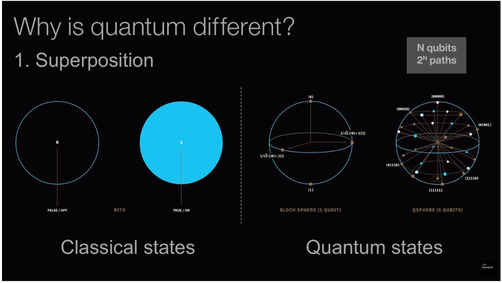
How to Measure the Unmeasurable: Explorations into Quantum Computing Readouts
I haven’t written much lately about Quantum Computing, not because it’s less interesting, just because I’ve been so preoccupied with all of the breakthroughs in the Artificial Intelligence research, that…
-

🔮 Unveiling the Hidden Magic: How a URL Transforms into a Webpage 🧙
Hello, dear readers! Today I’m going to explain one of the most basic and fascinating concepts of the web world: what happens when you navigate to a URL in a…
-

Quantum Computing and AI Tie the Knot
In 2018, quantum technicians and daring developers are using quantum algorithms to transform the field of artificial neural network optimization: the bees knees of machine learning and AI. So we…
-

Demystifying Quantum Gates — One Qubit At A Time
(I’ve written an introduction to quantum computing found here. If you are brand new to the field, it will be a better place to start.) If you want to get into…
-
The Need, Promise, and Reality of Quantum Computing
Despite giving us the most spectacular wave of technological innovation in human history, there are certain computational problems that the digital revolution still can’t seem to solve. Some of these…
-
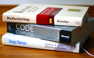
12 Most Influential Books Every Software Engineer Needs to Read
This is a question that I get a lot, especially from co-workers or friends that are just beginning their journey as a software craftsman. What book should I read to become…


